Return

CELLULAR AUTOMATA I HAVE KNOWN AND LOVED

Next |End This is the sort of book which should have been written by Alexander Shulgin, one of the most successful salesmen scientists of the twentieth century. Shulgin helped to research then popularise the drug called ecstacy or more internationally known as XTC. Any chemist will recognise the structural formulae for illegal drugs such as LSD or everyday chemicals such as the bases of DNA. So in information science the specifications of line automata can be written and recognised by different people in different parts of the world. Cellular automata are models used by scientists to describe the real world. Fibonacci's rabbits and Pascal's Triangle (known to Omar Khayyam) are examples of the output of Cellular Automata. The Sierpinski gasket is frequently referred to by mathematicians writing about Cantor's Ternary Set, but it crops up when the Pascal triangle or some Fibonacci style series are arranged in lines then coloured odd or even. A line automata can be specified with very simple rules. Stephen Wolfram described these in an article on the connections between mathematics and computer Science. This appeared in the Scientific American, in 1984. The definitions were accompanied by some very interesting pictures. One of them showed what might be green slimey stuff in a pond: surely a breeding ground for artificial life. The signature of this image could be written down (0131123). Any person with a computer can recreate this line automaton. The rules for line automata are simply explained in terms of vector mathematics where you work on rows of data. The line automaton is a generalisation of a finite state machine. The finite state machine is a computer science concept invented in the 1930s. The definition is very straightforward. A finite state machine is a collection of machine states S, input values I and response values R, along with two transition functions F and G. F: S x I -> S State transition function G: S x I -> R Response function The stimulus response nature of this model suggests an abstraction of Pavlov's dogs and behaviourist psychology. This definition is taken from Marvin Minsky's book "Finite & Infinite Machines". Marvin Minsky was a researcher at the Massachusetts Institute of Technology (MIT) and the book was a regular textbook for computer scientists in the late 1960s and early 1970s. In a line automaton finite state machines are arranged in a line, and inputs are the states of neighbouring cells. Other regular geometric arrangements may be used and they are generally known as CA or 'Cellular Automata'. If successive input and output states are arranged in a sequence which may be indexed by the set of positive and negative natural numbers along with a pair of responses equivalent to 'move left' and 'move right' then the device is called a Turing Machine.

SCHEMATIC OF A TURING MACHINE

Next | Back|Top|End o-----o |FSS | o--+--o v o--o--o--o--o--o--o--o--o--o--o--o--o--o--o--o--o--o- ... TAPE | 0| 1| 1| 0| 1| 0| 1| 1| 1| | | | | | | | | o__o__o__o__o__o__o__o__o__o__o__o__o__o__o__o__o__o_ ... Turing used this concept to chase up a solution to Hilbert's Tenth Problem. This is something to do with Diaphontine Equations, a part of human culture popularised in the number riddles of the Arabs and Greeks. Diaphontine equations seek whole number solutions for problems such as x^2+y^2=z^2. More details can be found in Marvin Minsky's book. Turing's theory is very abstract and does not make for easy reading.

SIXTEEN DIFFERENT LINE AUTOMATA

Next | Back|Top|End Restrict the number of states to just two values: 0 and 1 or 'ON' and 'OFF'. The input to each cell is the state of its neighbour to the left. There is no explicit response. The state transition function F: S x I -> S is a function from the set Z2 x Z2 to Z2, and there are 2^(2x2)=16 such functions. The behaviour of an array of cells can be modelled by algebra. For ease of computer representation most such arrays are modelled as loops where the rightmost element is identified with the leftmost element. If the values of the cells are stored in an array X and the transition function F:Z2 x Z2 is made to work on column vectors then the transition from one generation to the other can by written: X <- F(X, L X) where L is the left shift operator. In fact the function may be encoded as a set of sixteen values, and a lookup table can be used. Pairs of (x,y) of 0,1 values may also be encoded to the values 0 1 2 3 by the expression z=x+2y. The transition function being in the set Map (Z2xZ2, Z2) can be given a name from classical logic. These names are well known in computer science. They include AND, OR, IMPLIES, NOT, XOR for exclusive or, and EQUALS. The new values of the vector X can be computed, and successive generations may be printed on the screen. Here we use the XOR function. X<-LA_XOR N |Linear automaton using exclusive or. X<-_40t1 & N<-24 #ifndef"N" AA: (8r" ")," O"[X] | display line X<-(X+1mX)#mod 2 | transition rule ->(0<N--)/AA

XOR LINEAR CELLULAR AUTOMATON

|Next|Back|Top|End .......................................O ......................................OO .....................................O.O ....................................OOOO ...................................O...O ..................................OO..OO .................................O.O.O.O ................................OOOOOOOO ...............................O.......O ..............................OO......OO .............................O.O.....O.O ............................OOOO....OOOO ...........................O...O...O...O ..........................OO..OO..OO..OO .........................O.O.O.O.O.O.O.O ........................OOOOOOOOOOOOOOOO .......................O...............O ......................OO..............OO .....................O.O.............O.O ....................OOOO............OOOO ...................O...O...........O...O ..................OO..OO..........OO..OO .................O.O.O.O.........O.O.O.O ................OOOOOOOO........OOOOOOOO ...............O.......O.......O.......O ..............OO......OO......OO......OO .............O.O.....O.O.....O.O.....O.O ............OOOO....OOOO....OOOO....OOOO ...........O...O...O...O...O...O...O...O ..........OO..OO..OO..OO..OO..OO..OO..OO .........O.O.O.O.O.O.O.O.O.O.O.O.O.O.O.O ........OOOOOOOOOOOOOOOOOOOOOOOOOOOOOOOO 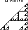Any person with access to a computer may experiment with cellular automata. Just like in any scientific enterprise the same results will be obtained by repeating the same experiments. Because of the simplicity of these experiments many different results may be obtained for different transition rules. An observant reader will see that the cellular automata gives Pscal's triangle reduced to even or odd. By an amazing coincidence of mathematics this form was given another name during the 1900s when mathematicians were defining Topology, or the business of how close things may be to each other. Cantor divided an interval into three then threw away the middle interval. He then repeated the process indefinately creating a copy of the unit interval within itself but occupying zero area. This lead to the mathematical theory of Surgery on Manifolds associated with Banach, Hausdorff and Sierpinski. Julia was also working in this area 100 years ago. The shape is called the 'Sierpinski Gasket' and it is often printed in books on fractals. Fractals may appear quite different from the evolution of cellular automata but in fact they are part of the same branch of mathematics. This is called 'Dynamical Systems Theory'. Needless to say Dynamical Systems were also invented over one hundred years ago, long before computers were ever invented. Poincare was one of the first mathematicians to write on the subject.

SIXTEEN IMAGES

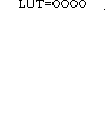
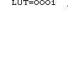
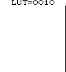
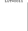
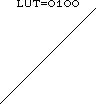
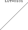
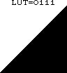
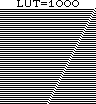
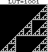
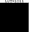
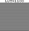
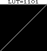
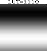
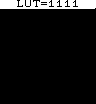
| Back|Top|End These represent the sixteen simplest possible line automata. Some people claim that similar growth patterns can model everything in the universe. Unlike many wild theories some of these results may be investigated and verified by anyone with access to a personal computer and any knowledge of any programming language. The algorithm for line cell J in line T is X[T+1,J] <- F (X[T,J], X[T,J-1]) where F is one of the sixteen possible logic functions on 0,1 pairs.