Return

This file was generated from sketch.txt

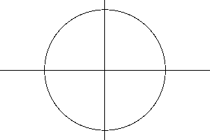
Curve sketching has been part of the mathematics syllabus for at least fifty years. Some people find this enjoyable, and they will try to sketch curves that the teachers do not necessarily talk about. Every student of mathematics will at some stage learn about a circle, and how to draw one. Any one who looks out of the window on a flight over arid regions will see the occassional circular patch of green. The radius of the circle is the length of the irrigation pipe which will be moved around, often by poorly paid migrant workers. This type of irrigation is called a 'Center Pivot' system.

The airline passenger will see all these perfect round shapes and may be very impressed, but some other curves are involved. The underground reservoir may have formed over thousands of years, and modern agricultural methods may deplete this in a short number of decades. It is possible to make a rough sketch of the amount of water in that reservoir, against time. The estimation of stuff in underground reservoirs is very tricky to calculate, and the results are often kept secret, so quite often the very best graph is nothing but a rough sketch. There are some important features of such a curve.

If the reservoir is replenished by rainfall, faster than it is used up, then the capacity will increase in time giving a positive slope. When replenishment and depletion are balanced there will be a zero slope, and when depletion exceeds replenishment the slope is negative. The negative slope may appear to be an almost vertical cliff. These types of cliffs are called discontinuities. In mathematics they are often expressed as conditional statements such as f(x)= ax if x less than t and f(x) = at-bx if x greater than t. The C-programming language also has a construction:

 y = (x < t) ? a*x : a*t-b*x; 

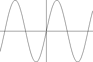
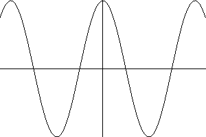
Other curves are found in text books. The parabola is quite common. The general equation is y=ax^2+bx+c and this equation may cross the x-axis at two points, just touch it, or turn away before crossing the axis. The differential coefficient dy/dx = 2ax+b will always be zero somewhere (at -b/2a) so there is always a maxinum or minimum. An example is y=4x(1-x). Here y is zero at x=0 and x=1, and a maximum at x=1/2. Values of x for which a function f(x)=0 are called roots of a function, or roots of the equation f(x)=0. The trigonometrical functions sin(x) and cos(x) have regularly spaced roots at values n*pi and (n+1/2)*pi. It is easy to see that these functions are essentially the same with just a shift along the x-axis needed to transform one into the other.

The sine function has maxima and minima where cosine is zero.

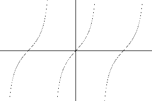
The tangent function has special problems. The definition tan(x)= sin(x)/cos(x) means that the function will become infinite whenever cos(x) =0, and this will happen quite often. The way do do this on the computer is the use of an implicit function. Find the (x,y) points which are zeros of a function z=F(x,y) where F is a function of two variables. Counting zeros of F(x,y) in a given zone does not require computing values where the function becomes infinity. When the points are sparse the computer graph may become invisible, but one of the advantages is that square roots are always given both positive and negative values.

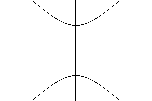
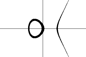
Two examples are given: a hyperbola y^2-x^2=1 and an elliptic curve y^2=x(x^2-1). The equation y^2-x^2=1 gives y^2=1+x^2, and there are no zeros for real values of x. The curve has two distinct parts.

These curves are always easier to do with a pencil and paper, rather than a computer. Mathematica retails for several hundred dollars and it can do symbolic calculus operations to find tangents, and radii of curvature. A biro and a few sheets of paper are affordable in much of the world, except Africa or Afghanistan. A kitchen table computer system such as the one which produced these sketches is available for the cost of a google search and download.

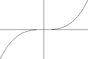
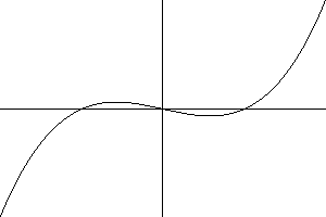
Two types of cubic may be seen. One has two distinct turning points while the other has only a flattening at one point. How a particular curve y=f(x) behaves can be deduced by examining the differential coefficient dy/dx = f'(x). For a cubic of the form y=x^3+ax+b this is f'(x)=3x^2+a with roots + or - sqrt(|a|/3) when a is negative.

For examples and definitions see Klaas Rover's teaching pages. There are also some linux tutorials.